Histograms of Oriented Gradients (HOG) 定向梯度直方图(HOG)
正如我们在ORB算法中看到的那样,我们可以使用图像中的关键点来进行基于关键点的匹配,以检测图像中的对象。 当您想要检测具有许多不受背景影响的一致内部特征的对象时,这些类型的算法非常有用。 例如,这些算法适用于面部检测,因为面部具有许多不受图像背景影响的一致内部特征,例如眼睛,鼻子和嘴巴。 然而,当尝试进行更一般的对象识别时,这些类型的算法不能很好地工作,例如,图像中的行人检测。 原因是人们没有像脸一样的内部特征,因为每个人的体形和风格都不同(见图1)。 这意味着每个人都将拥有不同的内部特征,因此我们需要一些可以更一般地描述一个人的东西。
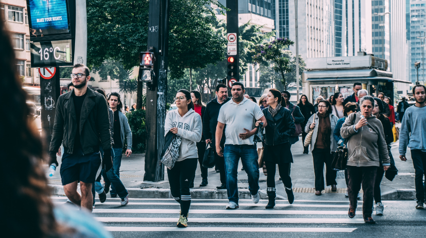
图1 行人
一种选择是尝试通过轮廓检测行人。 通过轮廓(边界)检测图像中的对象是非常具有挑战性的,因为我们必须处理由背景和前景之间的对比带来的困难。 例如,假设您想要检测在白色建筑物前行走的图像中的行人,并且她穿着白色外套和黑色裤子(参见图2)。 我们可以在图2中看到,由于图像的背景大部分是白色,因此黑色裤子将具有非常高的对比度,但是由于它也是白色的,因此具有非常低的对比度。 在这种情况下,检测裤子的边缘将是容易的,但检测外套的边缘将是非常困难的。 这就是** HOG 的用武之地.HOG代表直方图的直方图**,它是由Navneet Dalal和Bill Triggs于2005年首次推出的。

图2 高低对比度
HOG算法通过创建图像中梯度方向分布的直方图,然后以非常特殊的方式对它们进行标准化来工作。 即使在对比度非常低的情况下,这种特殊的标准化也使HOG在检测物体边缘时非常有效。 这些归一化的直方图被放在一个特征向量中,称为HOG描述符,可用于训练机器学习算法,例如支持向量机(SVM),以根据它们的边界(边缘)检测图像中的对象。。 由于其巨大的成功和可靠性,HOG已成为用于物体检测的计算机视觉中最广泛使用的算法之一。
在这个笔记本中,您将学到:
①HOG算法如何工作
②如何使用OpenCV创建HOG描述符
③如何可视化HOG描述符。
The HOG Algorithm
顾名思义,HOG算法基于从图像梯度的方向创建直方图。 HOG算法通过一系列步骤实现:
1.给定特定对象的图像,设置覆盖图像中整个对象的检测窗口(感兴趣的区域)(参见图3)。
2.计算检测窗口中每个像素的梯度大小和方向。
3.将检测窗口划分为连接的像素*单元格,所有单元格大小相同(参见图3)。单元格的大小是一个自由参数,通常选择它以匹配想要检测的特征的比例。例如,在64×128像素检测窗口中,6到8个像素宽的正方形单元适合于检测人体肢体。
4.为每个单元格创建直方图,首先将每个单元格中所有像素的渐变方向分组为特定数量的方向(角度)区域;然后将每个角度箱中梯度的梯度大小相加(见图3)。直方图中的区间数是一个自由参数,通常设置为9个角度区间。
5.将相邻单元分组为块*(参见图3)。每个块中的单元数是一个自由参数,所有块必须具有相同的大小。每个块之间的距离(称为步幅)是一个自由参数,但通常设置为块大小的一半,在这种情况下,您将获得重叠块(见下面的视频*)。已经凭经验显示HOG算法以更好地与重叠块一起工作。
6.使用每个块中包含的单元格来规范化该块中的单元格直方图(参见图3)。如果您有重叠块,这意味着大多数单元格将根据不同的块进行标准化(请参见下面的视频)。因此,相同的单元可以具有几种不同的标准化。
7.将所有块中的所有标准化直方图收集到称为HOG描述符的单个特征向量中。
8.使用来自相同类型对象的许多图像的结果HOG描述符来训练机器学习算法(例如SVM)以检测图像中的那些类型的对象。例如,您可以使用来自行人的许多图像的HOG描述符来训练SVM以检测图像中的行人。训练是通过您想要在图像中检测到的对象的正面负面示例完成的。
9.一旦训练了SVM,就会使用滑动窗口方法来尝试检测和定位图像中的对象。检测图像中的对象需要找到与SVM所学习的HOG图案类似的图像部分。

Fig. 3. - HOG Diagram.
为什么HOG算法有效
如上所述,HOG通过在图像的局部部分(称为* cells *)中添加特定方向的渐变幅度来创建直方图。通过这样做,我们保证更强的梯度将对其各自的角度仓的大小做出更多贡献,同时由噪声导致的弱和随机定向梯度的影响被最小化。以这种方式,直方图告诉我们每个细胞的主要梯度方向。
处理对比度
现在,由于局部照明的变化以及背景和前景之间的对比度,主导方向的大小可以广泛变化。
为了解释背景 - 前景对比度差异,HOG算法尝试在本地检测边缘。为了做到这一点,它定义了一组称为块**的单元格,并使用这个本地单元格组对直方图进行标准化。通过局部归一化,HOG算法可以非常可靠地检测每个块中的边缘;这称为块规范化**。
除了使用块规范化之外,HOG算法还使用重叠块来提高其性能。通过使用重叠块,每个单元向最终HOG描述符贡献若干独立分量,其中每个分量对应于相对于不同块标准化的单元。这似乎是多余的,但是,经验证明,通过相对于不同的本地块对每个小区进行几次归一化,HOG算法的性能显着提高。
加载图像和导入资源
构建我们的HOG描述符的第一步是将所需的包加载到Python中并加载我们的图像。
我们首先使用OpenCV加载三角形图块的图像。 因为cv2.imread()`函数将图像加载为BGR,我们将把图像转换为RGB,这样我们就可以用正确的颜色显示它。 像往常一样,我们会将BGR图像转换为Gray Scale进行分析。
import cv2
import numpy as np
import matplotlib.pyplot as plt


# Set the default figure size
plt.rcParams['figure.figsize'] = [17.0, 7.0]

# Load the image
image = cv2.imread('./images/triangle_tile.jpeg')

# Convert the original image to RGB
original_image = cv2.cvtColor(image, cv2.COLOR_BGR2RGB)

# Convert the original image to gray scale
gray_image = cv2.cvtColor(image, cv2.COLOR_BGR2GRAY)

# Print the shape of the original and gray scale images
print('The original image has shape: ', original_image.shape)
print('The gray scale image has shape: ', gray_image.shape)

# Display the images
plt.subplot(121)
plt.imshow(original_image)
plt.title('Original Image')
plt.subplot(122)
plt.imshow(gray_image, cmap='gray')
plt.title('Gray Scale Image')
plt.show()

创建HOG描述符
我们将使用OpenCV的HOGDescriptor类来创建HOG描述符。 使用HOGDescriptor()函数设置HOG描述符的参数。 HOGDescriptor()函数的参数及其默认值如下:
cv2.HOGDescriptor(win_size = (64, 128),
                  block_size = (16, 16),
                  block_stride = (8, 8),
                  cell_size = (8, 8),
                  nbins = 9,
                  win_sigma = DEFAULT_WIN_SIGMA,
                  threshold_L2hys = 0.2,
                  gamma_correction = true,
                  nlevels = DEFAULT_NLEVELS)
参数:
win_size - 大小
检测窗口的大小(以像素为单位)(宽度,高度)。定义感兴趣的区域。必须是单元格大小的整数倍。
block_size - 大小
块大小(以像素为单位)(宽度,高度)。定义每个块中有多少个单元格。必须是单元格大小的整数倍,并且必须小于检测窗口。块越小,您将获得更精细的细节。
block_stride - 大小
以像素为单位阻挡步幅(水平,垂直)。它必须是单元格大小的整数倍。 block_stride定义了adjecent块之间的距离,例如,水平8个像素和垂直8个像素。较长的block_strides使算法运行得更快(因为评估的块越少),但算法可能也不会运行。
cell_size - 大小
像素大小(宽度,高度)。确定细胞的大小。细胞越小,您将获得更精细的细节。
nbins - int
直方图的区间数。确定用于制作直方图的角度区间数。使用更多的垃圾箱可以捕获更多的渐变方向。 HOG使用无符号渐变,因此角度区间的值将介于0到180度之间。
win_sigma - double
高斯平滑窗口参数。通过在计算直方图之前对每个像素应用高斯空间窗口来平滑块边缘附近的像素,可以改善HOG算法的性能。
threshold_L2hys - double
L2-Hys(Lowe式限幅L2范数)归一化方法收缩。 L2-Hys方法用于归一化块,它由L2范数和剪切以及重新归一化组成。限幅将每个块的描述符向量的最大值限制为具有给定阈值的值(默认为0.2)。在剪辑之后,如IJCV,60(2):91-110,2004中所述,重新归一化描述符矢量。
gamma_correction - bool
用于指定是否需要伽马校正预处理的标志。执行伽马校正稍微提高了HOG算法的性能。
nlevels - int
检测窗口的最大数量增加。
我们可以看到,cv2.HOGDescriptor()函数支持各种参数。 前几个参数(block_size,block_stride,cell_size和nbins)可能是您最有可能更改的参数。 其他参数可以安全地保留其默认值,您将获得良好的结果。
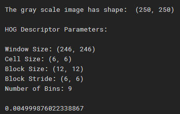
在下面的代码中,我们将使用cv2.HOGDescriptor()函数来设置单元格大小,块大小,块步幅以及HOG描述符直方图的bin数。 然后,我们将使用.compute(image)方法计算给定图像的HOG描述符(特征向量)。
# Specify the parameters for our HOG descriptor
# 指定HOG描述符的参数

# Cell Size in pixels (width, height). Must be smaller than the size of the detection window
# 以像素为单位的单元格大小(宽度, 高度),必须小于检测窗口的大小。
# and must be chosen so that the resulting Block Size is smaller than the detection window.
# 并且必须进行选择,以使所生成的块大小小于检测窗口的大小。
cell_size = (6, 6)

# Number of cells per block in each direction (x, y). Must be chosen so that the resulting
# Block Size is smaller than the detection window
# 每个方向(x,y)上每个块的单元数。必须进行选择,以使生成的块大小小于检测窗。
num_cells_per_block = (2, 2)

# Block Size in pixels (width, height). Must be an integer multiple of Cell Size.
# 以像素为为单位(宽,高)的块尺寸,必须是单元格大小的整数倍。
# The Block Size must be smaller than the detection window
# 块大小小于检测窗口的大小
block_size = (num_cells_per_block[0] * cell_size[0],
              num_cells_per_block[1] * cell_size[1])

# Calculate the number of cells that fit in our image in the x and y directions
# 计算单元格数量,以适应图像的x,y
x_cells = gray_image.shape[1] // cell_size[0]  #取整,比如:10//3==3
y_cells = gray_image.shape[0] // cell_size[1]

# Horizontal distance between blocks in units of Cell Size. Must be an integer and it must
# be set such that (x_cells - num_cells_per_block[0]) / h_stride = integer.
# 块之间的水平距离,以单元格大小为单位。必须是整数,且必须设置为:...
h_stride = 1

# Vertical distance between blocks in units of Cell Size. Must be an integer and it must
# be set such that (y_cells - num_cells_per_block[1]) / v_stride = integer.
v_stride = 1

# Block Stride in pixels (horizantal, vertical). Must be an integer multiple of Cell Size
# 块的步长,以像素为单位。必须是单元格尺寸的整数倍
block_stride = (cell_size[0] * h_stride, cell_size[1] * v_stride)

# Number of gradient orientation bins
# 梯度方向箱数量
num_bins = 9


# Specify the size of the detection window (Region of Interest) in pixels (width, height). 指定检测窗(ROI)的大小,以像素为单位。
# It must be an integer multiple of Cell Size and it must cover the entire image. Because  必须是单元格大小的整数倍,必须覆盖整个图像。
# the detection window must be an integer multiple of cell size, depending on the size of
# your cells, the resulting detection window might be slightly smaller than the image. 生成的检测窗可能略小于图像。
# This is perfectly ok. 这完全没有问题。
win_size = (x_cells * cell_size[0] , y_cells * cell_size[1])

# Print the shape of the gray scale image for reference
print('\nThe gray scale image has shape: ', gray_image.shape)
print()

# Print the parameters of our HOG descriptor
print('HOG Descriptor Parameters:\n')
print('Window Size:', win_size)
print('Cell Size:', cell_size)
print('Block Size:', block_size)
print('Block Stride:', block_stride)
print('Number of Bins:', num_bins)
print()

import time
time1 = time.time()

# Set the parameters of the HOG descriptor using the variables defined above
# 使用上面定义的变量,设置HOG描述符参数
hog = cv2.HOGDescriptor(win_size, block_size, block_stride, cell_size, num_bins)

# Compute the HOG Descriptor for the gray scale image
# 计算灰度图像的HOG描述符
hog_descriptor = hog.compute(gray_image)

print(time.time()-time1)
HOG描述符中的元素数量
得到的HOG描述符(特征向量)包含来自在一个长向量中连接的检测窗口中的所有块的所有单元的归一化直方图。 因此,HOG特征向量的大小将由检测窗口中的块总数乘以每个块的单元数乘以定向箱的数量来给出:

如果我们没有重叠块(即block_strideequals,block_size`),则可以通过将检测窗口的大小除以块大小来容易地计算块的总数。 但是,在一般情况下,我们必须考虑到我们有重叠块的事实。 要查找一般情况下的块总数(即*对于任何block_stride和block_size),我们可以使用下面给出的公式:
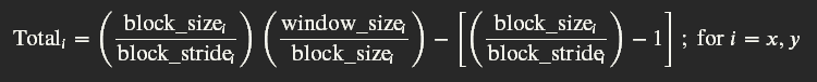
其中Total?x是沿检测窗口宽度的总块数,Total?y是沿检测窗口高度的块总数。 Total?x和Total?y的这个公式考虑了重叠产生的额外块。 在计算Total?x和Total?y之后,我们可以通过乘以Total?x××Total?来获得检测窗口中的块总数。 上面的公式可以大大简化,因为block_size,block_stride和window_size都是根据cell_size定义的。 通过进行所有适当的替换和取消,上述公式简化为:
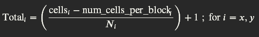
其中cells?x是沿检测窗口宽度的单元总数,而cells?y是沿检测窗口高度的单元总数。 并且??Nx是以cell_size为单位的水平块步幅,而??Ny是以cell_size为单位的垂直块步幅。
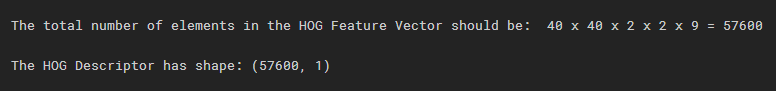
让我们计算HOG特征向量的元素数量,并检查它是否与上面计算的HOG描述符的形状相匹配。
# Calculate the total number of blocks along the width of the detection window  # 计算沿检测窗口宽度的块的总数
tot_bx = np.uint32(((x_cells - num_cells_per_block[0]) / h_stride) + 1)

# Calculate the total number of blocks along the height of the detection window
tot_by = np.uint32(((y_cells - num_cells_per_block[1]) / v_stride) + 1)

# Calculate the total number of elements in the feature vector  计算特征向量中元素的总数
tot_els = (tot_bx) * (tot_by) * num_cells_per_block[0] * num_cells_per_block[1] * num_bins

# Print the total number of elements the HOG feature vector should have  打印HOG特征向量应具有的元素总数
print('\nThe total number of elements in the HOG Feature Vector should be: ',
      tot_bx, 'x',
      tot_by, 'x',
      num_cells_per_block[0], 'x',
      num_cells_per_block[1], 'x',
      num_bins, '=',
      tot_els)

# Print the shape of the HOG Descriptor to see that it matches the above #打印HOG描述符的形状,看它是否符合上述要求。
print('\nThe HOG Descriptor has shape:', hog_descriptor.shape)
print()
可视化HOG描述符
我们可以通过将与每个细胞相关联的直方图绘制为矢量集合来可视化HOG描述符。为此,我们将直方图中的每个bin绘制为单个向量,其大小由bin的高度给出,其方向由与其关联的角度bin给出。由于任何给定的单元格可能有多个与之关联的直方图,由于重叠的块,我们将选择平均每个单元格的所有直方图,以便为每个单元格生成单个直方图。
OpenCV没有简单的方法可视化HOG描述符,因此我们必须先进行一些操作才能使其可视化。我们将从重塑HOG描述符开始,以便使我们的计算更容易。然后我们将计算每个单元的平均直方图,最后我们将直方图箱转换为矢量。一旦我们有了矢量,我们就会为图像中的每个细胞绘制相应的矢量。
下面的代码生成一个交互式绘图,以便您可以与图形进行交互。该图包含: *灰度图像,
- HOG描述符(特征向量),
- HOG描述符的放大部分,和 *所选单元格的直方图。
您可以单击灰度图像或HOG描述符图像上的任意位置以选择特定单元格。单击任一图像后,将出现* magenta *矩形,显示您选择的单元格。缩放窗口将显示所选单元格周围的HOG描述符的放大版本;直方图将显示所选单元格的相应直方图。交互式窗口底部还有按钮,允许其他功能,例如平移,并根据需要为您提供保存图形的选项。主页按钮将图形返回到其默认值。
注意:如果您在Udacity工作区中运行此笔记本,则交互式绘图中会有大约2秒的延迟。这意味着如果单击图像进行放大,则图表刷新大约需要2秒钟。
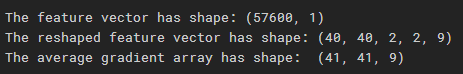
%matplotlib notebook

import copy
import matplotlib.patches as patches

# Set the default figure size
plt.rcParams['figure.figsize'] = [9.8, 9]

# Reshape the feature vector to [blocks_y, blocks_x, num_cells_per_block_x, num_cells_per_block_y, num_bins].
# The blocks_x and blocks_y will be transposed so that the first index (blocks_y) referes to the row number
# and the second index to the column number. This will be useful later when we plot the feature vector, so
# that the feature vector indexing matches the image indexing.
hog_descriptor_reshaped = hog_descriptor.reshape(tot_bx,
                                                 tot_by,
                                                 num_cells_per_block[0],
                                                 num_cells_per_block[1],
                                                 num_bins).transpose((1, 0, 2, 3, 4))

# Print the shape of the feature vector for reference
print('The feature vector has shape:', hog_descriptor.shape)

# Print the reshaped feature vector
print('The reshaped feature vector has shape:', hog_descriptor_reshaped.shape)

# Create an array that will hold the average gradients for each cell
ave_grad = np.zeros((y_cells, x_cells, num_bins))

# Print the shape of the ave_grad array for reference
print('The average gradient array has shape: ', ave_grad.shape)

# Create an array that will count the number of histograms per cell
hist_counter = np.zeros((y_cells, x_cells, 1))

# Add up all the histograms for each cell and count the number of histograms per cell
for i in range (num_cells_per_block[0]):
    for j in range(num_cells_per_block[1]):
        ave_grad[i:tot_by + i,
                 j:tot_bx + j] += hog_descriptor_reshaped[:, :, i, j, :]

        hist_counter[i:tot_by + i,
                     j:tot_bx + j] += 1

# Calculate the average gradient for each cell
ave_grad /= hist_counter

# Calculate the total number of vectors we have in all the cells.
len_vecs = ave_grad.shape[0] * ave_grad.shape[1] * ave_grad.shape[2]

# Create an array that has num_bins equally spaced between 0 and 180 degress in radians.
deg = np.linspace(0, np.pi, num_bins, endpoint = False)

# Each cell will have a histogram with num_bins. For each cell, plot each bin as a vector (with its magnitude
# equal to the height of the bin in the histogram, and its angle corresponding to the bin in the histogram).
# To do this, create rank 1 arrays that will hold the (x,y)-coordinate of all the vectors in all the cells in the
# image. Also, create the rank 1 arrays that will hold all the (U,V)-components of all the vectors in all the
# cells in the image. Create the arrays that will hold all the vector positons and components.
U = np.zeros((len_vecs))
V = np.zeros((len_vecs))
X = np.zeros((len_vecs))
Y = np.zeros((len_vecs))

# Set the counter to zero
counter = 0

# Use the cosine and sine functions to calculate the vector components (U,V) from their maginitudes. Remember the
# cosine and sine functions take angles in radians. Calculate the vector positions and magnitudes from the
# average gradient array
for i in range(ave_grad.shape[0]):
    for j in range(ave_grad.shape[1]):
        for k in range(ave_grad.shape[2]):
            U[counter] = ave_grad[i,j,k] * np.cos(deg[k])
            V[counter] = ave_grad[i,j,k] * np.sin(deg[k])

            X[counter] = (cell_size[0] / 2) + (cell_size[0] * i)
            Y[counter] = (cell_size[1] / 2) + (cell_size[1] * j)

            counter = counter + 1

# Create the bins in degress to plot our histogram.
angle_axis = np.linspace(0, 180, num_bins, endpoint = False)
angle_axis += ((angle_axis[1] - angle_axis[0]) / 2)

# Create a figure with 4 subplots arranged in 2 x 2
fig, ((a,b),(c,d)) = plt.subplots(2,2)

# Set the title of each subplot
a.set(title = 'Gray Scale Image\n(Click to Zoom)')
b.set(title = 'HOG Descriptor\n(Click to Zoom)')
c.set(title = 'Zoom Window', xlim = (0, 18), ylim = (0, 18), autoscale_on = False)
d.set(title = 'Histogram of Gradients')

# Plot the gray scale image
a.imshow(gray_image, cmap = 'gray')
a.set_aspect(aspect = 1)

# Plot the feature vector (HOG Descriptor)
b.quiver(Y, X, U, V, color = 'white', headwidth = 0, headlength = 0, scale_units = 'inches', scale = 5)
b.invert_yaxis()
b.set_aspect(aspect = 1)
b.set_facecolor('black')

# Define function for interactive zoom
def onpress(event):

    #Unless the left mouse button is pressed do nothing
    if event.button != 1:
        return

    # Only accept clicks for subplots a and b
    if event.inaxes in [a, b]:

        # Get mouse click coordinates
        x, y = event.xdata, event.ydata

        # Select the cell closest to the mouse click coordinates
        cell_num_x = np.uint32(x / cell_size[0])
        cell_num_y = np.uint32(y / cell_size[1])

        # Set the edge coordinates of the rectangle patch
        edgex = x - (x % cell_size[0])
        edgey = y - (y % cell_size[1])

        # Create a rectangle patch that matches the the cell selected above
        rect = patches.Rectangle((edgex, edgey),
                                  cell_size[0], cell_size[1],
                                  linewidth = 1,
                                  edgecolor = 'magenta',
                                  facecolor='none')

        # A single patch can only be used in a single plot. Create copies
        # of the patch to use in the other subplots
        rect2 = copy.copy(rect)
        rect3 = copy.copy(rect)

        # Update all subplots
        a.clear()
        a.set(title = 'Gray Scale Image\n(Click to Zoom)')
        a.imshow(gray_image, cmap = 'gray')
        a.set_aspect(aspect = 1)
        a.add_patch(rect)

        b.clear()
        b.set(title = 'HOG Descriptor\n(Click to Zoom)')
        b.quiver(Y, X, U, V, color = 'white', headwidth = 0, headlength = 0, scale_units = 'inches', scale = 5)
        b.invert_yaxis()
        b.set_aspect(aspect = 1)
        b.set_facecolor('black')
        b.add_patch(rect2)

        c.clear()
        c.set(title = 'Zoom Window')
        c.quiver(Y, X, U, V, color = 'white', headwidth = 0, headlength = 0, scale_units = 'inches', scale = 1)
        c.set_xlim(edgex - cell_size[0], edgex + (2 * cell_size[0]))
        c.set_ylim(edgey - cell_size[1], edgey + (2 * cell_size[1]))
        c.invert_yaxis()
        c.set_aspect(aspect = 1)
        c.set_facecolor('black')
        c.add_patch(rect3)

        d.clear()
        d.set(title = 'Histogram of Gradients')
        d.grid()
        d.set_xlim(0, 180)
        d.set_xticks(angle_axis)
        d.set_xlabel('Angle')
        d.bar(angle_axis,
              ave_grad[cell_num_y, cell_num_x, :],
              180 // num_bins,
              align = 'center',
              alpha = 0.5,
              linewidth = 1.2,
              edgecolor = 'k')

        fig.canvas.draw()

# Create a connection between the figure and the mouse click
fig.canvas.mpl_connect('button_press_event', onpress)
plt.show()

了解直方图
让我们看一下上图的几个快照,看看所选单元格的直方图是否有意义。 让我们开始查看三角形内部而不是边缘附近的单元格:
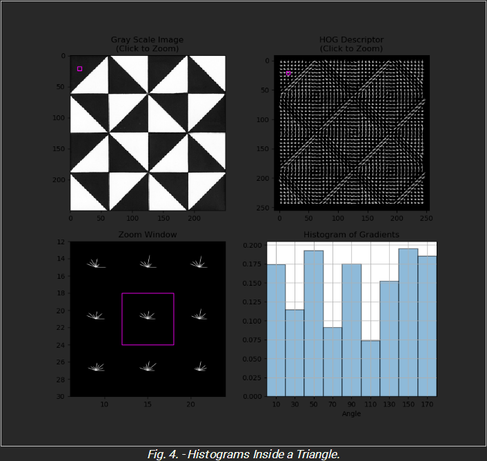
在这种情况下,由于三角形几乎都是相同的颜色,因此在所选单元格中不应存在任何主要梯度。 正如我们在缩放窗口和直方图中可以清楚地看到的那样,情况确实如此。 我们有很多渐变但没有一个明显地支配着另一个。 现在让我们看一下靠近水平边缘的单元格

请记住,边缘是图像中强度突然变化的区域。 在这些情况下,我们将在某个特定方向上具有高强度梯度。 这正是我们在所选单元格的相应直方图和缩放窗口中看到的内容。 在缩放窗口中,我们可以看到主导梯度向上,几乎在90度,因为这是强度急剧变化的方向。 因此,我们应该期望直方图中的90度区域比其他区域更强。 这实际上就是我们所看到的。 现在让我们看一下靠近垂直边缘的单元格:

在这种情况下,我们期望单元格中的主导梯度是水平的,接近180度,因为这是强度急剧变化的方向。 因此,我们应该期望直方图中的170度区域比其他区域强烈支配。 这就是我们在直方图中看到的,但我们也看到细胞中还有另一个显性梯度,即10度箱中的梯度。 原因是因为HOG算法使用无符号梯度,这意味着0度和180度被认为是相同的。 因此,当创建直方图时,160度和180度之间的角度与10度箱和170度箱成比例。 这导致在垂直边缘附近的单元中存在两个主要梯度而不是仅一个。 总结一下,让我们看一下靠近对角线边缘的单元格。

为了理解我们所看到的,让我们首先记住渐变有一个* x * - 组件和一个* y * - 组件,就像矢量一样。因此,梯度的最终方向将由其分量的矢量和给出。因此,在垂直边缘上,渐变是水平的,因为它们只有x分量,如图4所示。在水平边缘上,渐变是垂直的,因为它们只有y分量,正如我们在图3.因此,在对角线边缘,梯度也将是对角线,因为* x 和 y *分量都是非零的。由于图像中的对角线边缘接近45度,我们应该期望在50度箱中看到显着的梯度方向。这实际上是我们在直方图中看到的,但是,如图4所示,我们看到有两个主导梯度而不是一个。其原因在于,当创建直方图时,靠近区间边界的角度与相邻区间成比例地贡献。例如,角度为40度的渐变位于30度和50度箱的中间。因此,梯度的大小均匀地分成30度和50度的箱。这导致在对角线边缘附近的单元中存在两个主要梯度而不是仅一个。
现在您已了解HOG的实现方式,在工作区中您将找到名为* Examples *的笔记本。在那里,您将能够为各种图像的HOG描述符设置自己的参数。玩得开心!